Introduction

Reading The Little Book of Common Sense Investing by John C. Bogle was an eye-opener for me. It made me realize that constructing a personal ETF portfolio isn’t as complex as it seems, and the results I achieve might not differ much from those of highly-paid professionals. Over the past few months, I’ve become increasingly convinced that I need to take control of my retirement savings, especially considering my skepticism about the future stability of nations over the next 30 years.

Additionally, after delving into Bitcoin and the Austrian School of Economics, I’ve come to understand that in our Keynesian economy, money cannot simply be saved passively—it requires active management. With this in mind, I’m embarking on a new chapter in my financial journey, preparing to manage my savings effectively. Let’s dive into the details!

Currency Selection

Before we explore my ETF choices, it’s important to first consider the currencies in which I’ll be investing:

• Euro (EUR):
  • As I plan to live in Europe, I want a slightly higher exposure to the euro, a strategy known as country bias. This has advantages like tax benefits and reduced currency risk. However, I’m mindful of not overexposing myself to the euro, given the European Central Bank’s dependence on U.S. economic policies.
• U.S. Dollar (USD):
  • The U.S. dollar is currently the world’s primary reserve currency, so it makes sense to allocate a portion of my portfolio to it. However, with the rise of the BRICS nations and their efforts to develop alternative monetary systems, I want my portfolio to be robust enough to weather any shifts away from the U.S. dollar’s dominance.
• Swiss Franc (CHF):
  • The Swiss franc is an excellent hedge against monetary inflation and offers diversification since it’s less tied to the U.S. economy. I also have plans to work remotely in Switzerland, so having some exposure to the franc aligns with my future income prospects.
• Gold:
  • While not a conventional currency, gold has long been a reliable store of value. Its non-inflationary nature makes it a crucial component of my portfolio. To me, gold is the only “real money” since fiat currencies are just pieces of paper that, for now, are recognized as legal tender, but they lack intrinsic value.

ETF Selection

All the ETFs I’ve chosen are accumulation-based, meaning they reinvest dividends, which is beneficial for tax efficiency and maximizing compounding. When selecting ETFs, I focused on two main criteria: Total Expense Ratio (TER) and fund capitalization.

1. Total Expense Ratio (TER): This is crucial for long-term investing, as high fees can erode the compounding effect over time. Therefore, I aimed to keep the TER as low as possible.
2. Fund Capitalization: I believe in market efficiency, so I opted for well-established ETFs with high liquidity and low spreads rather than exotic options with higher TERs.

• Vanguard S&P 500 UCITS ETF (USD):
  • This ETF provides broad exposure to the U.S. market, particularly in the IT and financial sectors, which together make up 44.8% of the fund.
• Xtrackers EURO STOXX 50 UCITS ETF (EUR):
  • Offering diversified exposure to European markets, this ETF is balanced across various sectors and doesn’t overly rely on the IT sector.
• UBS MSCI Switzerland 20/35 UCITS ETF (CHF):
  • Focused on Swiss markets, this ETF includes stable sectors like healthcare, financials, and consumer staples. It serves as a hedge against potential geopolitical risks.
• Xtrackers MSCI Emerging Markets (USD):
  • Given the growing influence of BRICS nations, I believe emerging markets will play a significant role in the future, making this ETF a necessary component of my portfolio.
• iShares MSCI Pacific ex Japan (USD):
  • This ETF gives me exposure to Australia and Hong Kong, regions with strong economic growth and abundant resources.
• Invesco Gold:
  • Instead of holding physical gold, which can be risky, I opted for this ETF that tracks the price of gold, offering a secure and convenient alternative.

If you’re interested in exploring these ETFs further, you can easily check them out on JustETF by clicking on the names in the list above.

Portfolio Composition

I structured my portfolio based on my preferred currency exposure:

• USD: 40%
• EUR: 20%
• CHF: 20%
• Gold: 20%

This led to the following allocation:

• Vanguard S&P 500 (USD): 20%
• Xtrackers MSCI Emerging Markets (USD): 10%
• MSCI Pacific ex Japan (USD): 10%
• Xtrackers EURO STOXX 50 (EUR): 20%
• UBS MSCI Switzerland 20/35 (CHF): 20%
• Invesco Gold (Gold): 20%

Fees Evaluation

Fees were a key factor in my ETF selection. Over a long time horizon, high fees can significantly diminish the benefits of compounding returns. While I sometimes chose ETFs with slightly higher spreads, I aimed to strike a balance by selecting well-known ETFs with lower overall costs.

ETF	Management fee	Transaction fee	Total fee
S&P 500	0.07 %	0.02 %	0.09 %
STOXX 50	0.09 %	0.01 %	0.10 %
MSCI Pacific ex Japan	0.20 %	0.02 %	0.22 %
MSCI Switzerland 20/35	0.20 %	0.00 %	0.20 %
MSCI Emerging Markets	0.18 %	0.03 %	0.21 %
Gold	0.12 %	0.00 %	0.12 %

Country and Sector Exposure

My goal with this portfolio is to create a balanced, long-term investment strategy. Historical performance is not always a reliable indicator of future returns, especially given the potential rise of BRICS and the shifting global economic landscape. Therefore, I’ve diversified across regions and sectors to mitigate risks.

Sector Exposure:
I categorized sectors into three groups:

• Speculative Sectors: IT, financials, energy, and consumer discretionary—volatile but often profitable during economic growth.
• Stable Sectors: Industrials, healthcare, consumer staples, and utilities—these provide steady returns across different economic cycles.
• Recession-Resistant Sectors: Communication services, materials, and real estate—more stable during economic downturns.

Country Exposure:
I intentionally reduced my reliance on the U.S., with only 20% of my portfolio in U.S. equities. Europe and Switzerland each also have 20%, with the remaining 20% diversified across emerging markets, including China, Australia, India, Taiwan, Singapore, and Hong Kong.

ETF Correlation

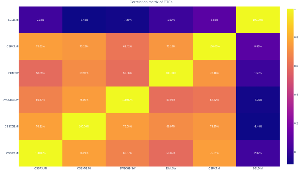
The ETFs in my portfolio exhibit correlations ranging from 60% to 80%, with gold being nearly independent. This indicates that my portfolio is reasonably diversified, reducing the risk of significant losses during market downturns.

Past Performance Analysis

As someone who enjoys math and simulations, I couldn’t resist diving into the historical data. However, it’s important to emphasize that the results presented here are not necessarily indicative of future performance. Markets are unpredictable, and past performance does not guarantee future results. With that caveat in mind, let’s explore the simulation.

All computations can also be found in the GitHub repository!

Simulation Objective

The goal was to estimate the portfolio’s annualized average returns and volatility, along with the 95% credible interval for these metrics.

Historical Data Analysis

To start, I used actual historical data to compute the portfolio’s average annual return and volatility. This was achieved by applying the covariance matrix and the ETF weights.

• Portfolio Annual Volatility: 12.93%
• Portfolio Annual Return: 8.96%

Normality Check

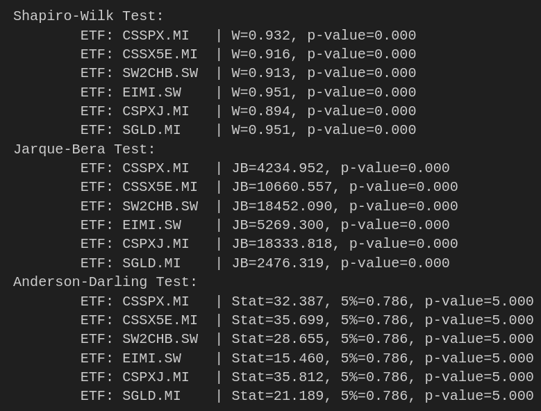
To assess whether the distribution of returns for each ETF is normally distributed, I conducted three statistical tests: Shapiro-Wilk, Jarque-Bera, and Anderson-Darling. The results from all three tests indicated that none of the ETFs follows a normal distribution. Given this, I chose to proceed with the analysis using a Monte Carlo simulation approach, which doesn’t rely on the assumption of normality.

Monte Carlo Simulation

I ran a Monte Carlo simulation by generating 10,000 series of returns, each obtained by randomly sampling with replacement from the original return series. Using these simulated datasets, I calculated the average returns and volatility. The results, presented with a 95% credible interval, are as follows:

• Annualized Mean Returns: [0.96% : 16.92%]
• Annualized Volatility: [11.97% : 13.98%]

These results suggest that while the portfolio is expected to have relatively low volatility compared to the S&P 500, it remains well-balanced.

Portfolio Simulation

• DCA Strategy: I simulated a scenario where €600 is invested each month from November 27, 2014, to the present.
• Lump-Sum Investing: In this scenario, €70,800 (the total amount invested in the DCA strategy) is invested in one go on the first day.

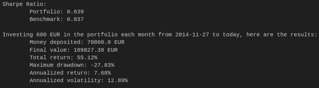
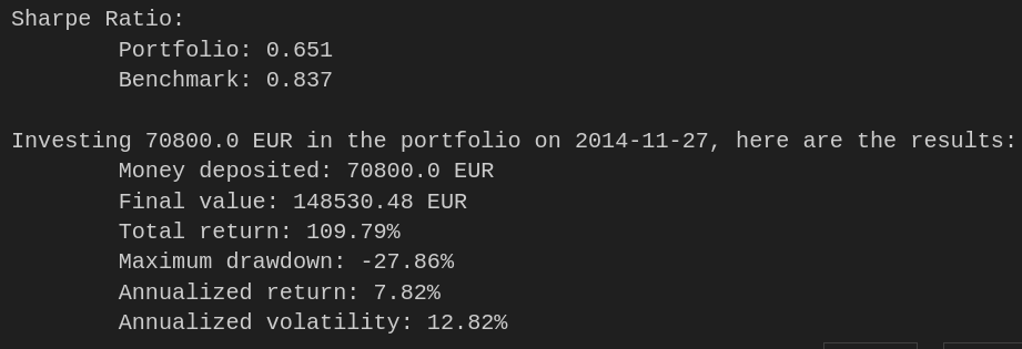
Results:
The lump-sum investment strategy significantly outperformed the DCA strategy over the long term. However, DCA remains the only viable option for investors who don’t have access to a large amount of capital upfront. In my case, the choice is to gradually invest through DCA, accepting that this approach might lead to lower potential gains compared to a lump-sum investment.

Key Considerations

While the historical performance of this portfolio may not match that of the S&P 500, there are important factors to consider:

1. Uncertain Future: As emphasized earlier, past performance is not a reliable indicator of future results.
2. Geopolitical Factors: This portfolio is designed to be resilient to geopolitical shifts, such as the rise of BRICS nations.
3. Market Dynamics: U.S. stocks may currently be overvalued due to the large volume of money in Western economies. This could change in the future.
4. Valuation of Emerging Markets: Emerging market stocks, while riskier, are often undervalued, presenting potential opportunities.
5. Balanced Approach: Chasing the highest past performance is rarely a good strategy. Instead, the focus should be on building a robust portfolio that can weather various future scenarios.

Conclusion

In summary, while my portfolio may not outperform the S&P 500 in the short term, it’s designed to be resilient against geopolitical shifts and the potential rise of emerging markets. I’m satisfied with the balance between risk and reward and will begin dollar-cost averaging (DCA) into this portfolio using a fee-free broker like Scalable Capital.

I understand that this portfolio isn’t perfect and that adjustments may be necessary over time. However, I believe that taking action now, even if imperfect, is better than waiting indefinitely for the “perfect” solution that may never come.